Benchmarking
A comprehensive comparison between multiple machine learning (ML) algorithms comprises
a thorough cross-validation of their predictive performance, this is known as Benchmarking.
You can quickly benchmark multiple algorithms such as Silverkite and Prophet using
the BenchmarkForecastConfig class.
The Benchmark class requires 3 inputs.
df : `pandas.DataFrame`
    Timeseries data to forecast.
    Contains columns [`time_col`, `value_col`], and optional regressor columns.
    Regressor columns should include future values for prediction.

configs : `Dict` [`str`,  `ForecastConfig`]
    Dictionary of model configurations.
    A model configuration is a member of the class
    `~greykite.framework.templates.autogen.forecast_config.ForecastConfig`.

tscv : `~greykite.sklearn.cross_validation.RollingTimeSeriesSplit`
    Cross-validation object that determines the rolling window evaluation.
    See :class:`~greykite.sklearn.cross_validation.RollingTimeSeriesSplit` for details.
In the sections we below provide guidance on how to design a proper cross-validation schema for your use case and discuss the structure of the benchmark output. Check the Benchmarking tutorial to learn the step-by-step process of defining and running a benchmark.
Rolling Window Cross-Validation (CV)
Time-series forecast quality strongly depends on the evaluation time window.
Thus it is more robust to evaluate over a longer time window when dataset size allows.
You can easily define the evaluation time window by using
RollingTimeSeriesSplit class.
See how in the Define the CV
section of the tutorial.
We use a rolling window CV for our benchmarking, which closely resembles the well known K-fold CV method. In K-fold CV, the original data is randomly partitioned into K equal sized subsamples. A single subsample is held out as the validation data, and the model is trained on the remaining (K-1) subsamples. The trained model is used to predict on the held-out validation set. This process is repeated K times so that each of the K subsamples is used exactly once as the validation set. Average testing error across all the K iterations provides an unbiased estimate of the true testing error of the machine learning (ML) model on the data.
Due to the temporal dependency in time-series data the standard K-fold CV is not appropriate. Choosing a hold-out set randomly has two fundamental issues in the timeseries context:
Future data is utilized to predict the past.
Some timeseries models can not be trained realistically with a random sample, e.g. the autoregressive models due to missing lags.
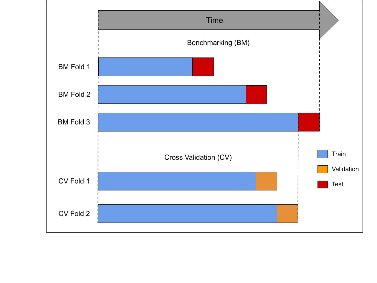
Rolling window CV addresses this by creating a series of K test sets, as illustrated in the previous Figure. For each test set, the observations prior to the test set are used for training. This creates K benchmark (BM)-folds. Within each training set, a series of CV folds is created, each containing a validation set. The number of datapoints in every test and validation set equals the forecast horizon. Observations that occur prior to that of the validation set are used to train the models for the corresponding CV fold. Thus, no future observations can be used in constructing the forecast, either in the validation or testing phase. The parameters minimizing average error on the validation sets are chosen. This model is then retrained on the training data for the corresponding BM-fold. The average error across all test sets provides a robust estimate of the model performance with this forecast horizon.
Selecting CV parameters
We provide a set of defaults for 3 different forecast horizons for hourly, daily and weekly datasets. These horizons roughly represent short-term, average-term and long-term forecasts for the corresponding frequency (e.g. 1 day, 7 day and 90 day ahead forecasts for daily data). The datasets must have at least 2 years worth of training data for the models to accurately estimate yearly seasonality patterns. These defaults provide a consistent benchmarking setting suitable for all algorithms, including the slower ones. The values are chosen based on the following principles:
The predictive performance of the models are measured over an year to ensure that cumulatively the test sets represent real data across time properties e.g. seasonality, holidays etc. For daily data,
periods between splits(25) *number of splits(16) = 400 > 365, hence the models are tested over a year.The test sets are completely randomized in terms of time features. For daily data, setting
periods between splitsto any multiple of 7 results in the training and test sets always ending on the same day of the week. This lack of randomization produce a biased estimate of the prediction performance. Similarly setting it to a multiple of 30 has the same problem for day of month. A gap of 25 days between test sets ensures that no such confounding factors are present.Minimize total computation time while maintaining the previous points. For daily data, setting
periods between splitsto 1 andnumber of splitsto 365 is a more thorough CV procedure. But it massively increases the total computation time and hence is avoided.
Frequency |
Forecast horizon |
CV horizon |
CV minimum train periods |
Periods between splits |
Number of splits |
|---|---|---|---|---|---|
hourly |
1 |
1 |
24 * 365 * 2 |
(24 * 24) + 7 |
16 |
hourly |
24 |
24 |
24 * 365 * 2 |
(24 * 24) + 7 |
16 |
hourly |
24 * 7 |
24 * 7 |
24 * 365 * 2 |
(24 * 24) + 7 |
16 |
daily |
1 |
1 |
365 * 2 |
25 |
16 |
daily |
7 |
7 |
365 * 2 |
25 |
16 |
daily |
90 |
90 |
365 * 2 |
25 |
16 |
weekly |
1 |
1 |
52 * 2 |
3 |
18 |
weekly |
4 |
4 |
52 * 2 |
3 |
18 |
weekly |
4 * 3 |
4 * 3 |
52 * 2 |
3 |
18 |
Note
The default parameters in the table provide a guideline for a sound CV procedure. The users are encouraged to modify it according to their needs as long as it adheres to the core principle. For example, if all the benchmarking models execute quickly, the values of
periods between splitsandnumber of splitscan be swapped for a more thorough benchmarking.
Monitoring the Benchmark
During benchmarking a couple of color coded progress bars are displayed to inform the user of the
advancement of the entire process. The first bar displays config level information, while
the second bar displays split level information for the current config.
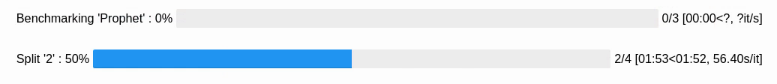
On the left side of the progress bar, it shows which config/ split is currently being
benchmarked and progress within that level as a percentage.
On the right side, the user can see how many configs/ splits have been benchmarked
and how many are remaining. Additionally, this bar also displays elapsed time and remaining runtime
for the corresponding level.
Note
The
configsand differentsplitswithin aconfigare run sequentially, however any cross-validation within asplitis parallelized. This ensures that the CPU cores are not overloaded and we can estimate the runtime accurately.
Output of the Benchmark
The output of a successful benchmark procedure is stored under the class attribute result
as a nested dictionary. Every node in the tree is a dictionary key.
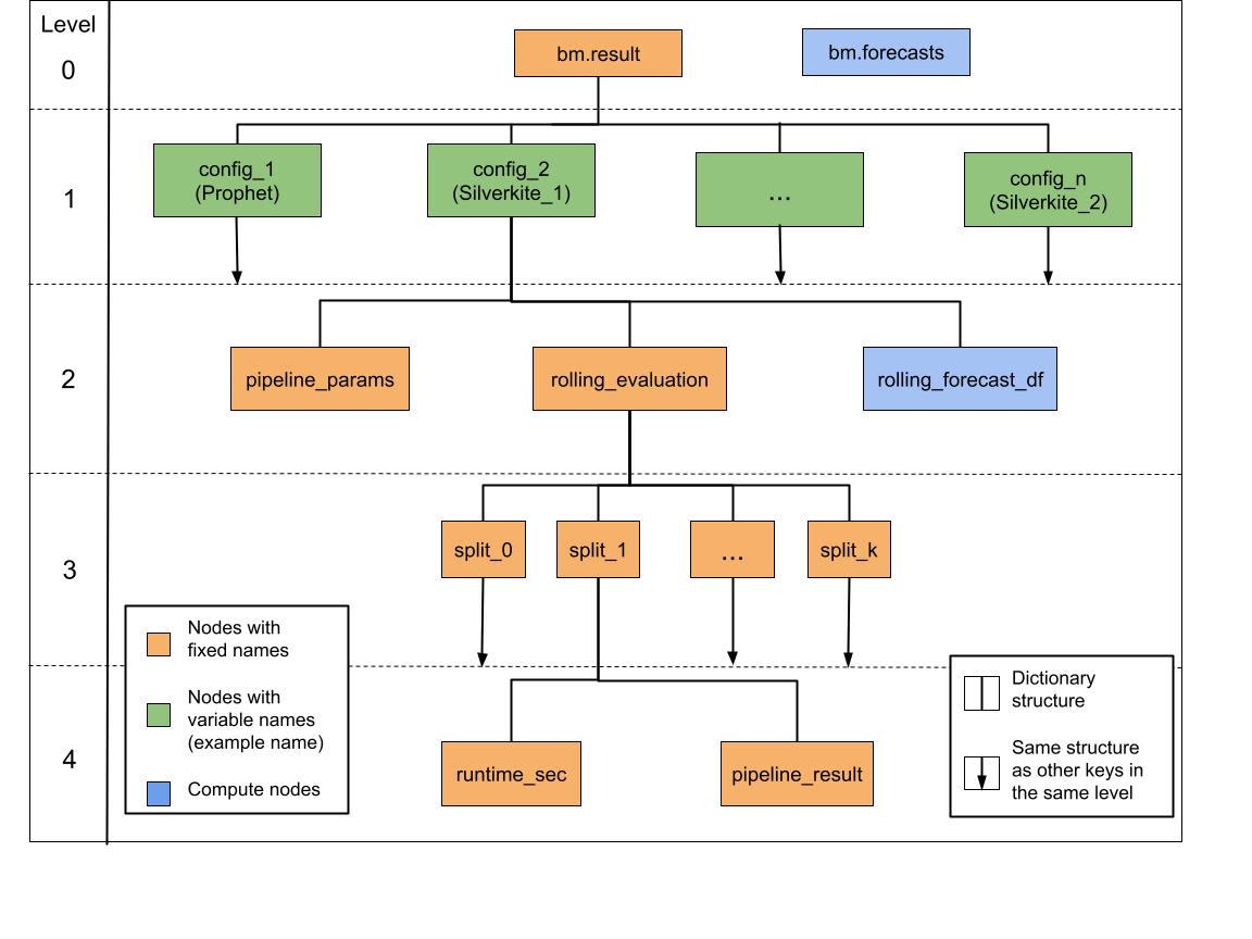
A compute node (node in blue) is a node that is computed only when the user specifically requests for the output. Here is a brief overview of the leaf nodes i.e. nodes without any link to the next level.
bm.forecasts : `pandas.DataFrame`
    Splitwise forecast output of all ``configs``.
    Helps in comparing forecasts and prediction accuracy across ``configs``.
    This node is computed when ``extract_forecasts`` method is run.

pipeline_params : `dict`
    Inputs to the
    `~greykite.framework.pipeline.pipeline.ForecastResult.forecast_pipeline`.
    Useful for debugging errors thrown by the ``validate`` method.

rolling_forecast_df : `pandas.DataFrame`
    Splitwise forecast output of the corresponding ``config``.
    Helps in comparing forecasts and prediction accuracy across splits.
    This node is computed when ``extract_forecasts`` method is run.

runtime_sec : `float`
    Runtime of the corresponding split of the ``config`` in seconds.

pipeline_result : `~greykite.framework.pipeline.pipeline.ForecastResult`
    Forecast output of the corresponding split of the ``config``.
Using the output you can quickly compute and visualize the prediction errors for multiple metrics. For examples check the Benchmark output section of the tutorial.